Due to a server crash, this webpage was unavailable for the past two days.
For some reason, both the mainboard and hard disk broke down. There was a recent backup, hence nothing of serious importance was lost.
Due to a server crash, this webpage was unavailable for the past two days.
For some reason, both the mainboard and hard disk broke down. There was a recent backup, hence nothing of serious importance was lost.
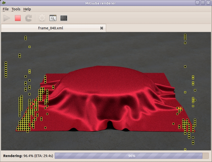
Every once in a while, I need to create an image that truly takes a very long time to render in Mitsuba, to the point that I am simply not willing to wait that long. In some cases, this just means that an inefficient algorithm somewhere in the code had better be replaced. But in other cases, the algorithms are all fine, and it’s really the scene’s fault for being excessively complicated. Such circumstances leave me with only two choices: 1. I can adjust my expectations and simplify the scene, or 2. throw a huge amount of processing power behind Mitsuba, and make it go fast. In this blog entry, I will explain how to do the latter with the help of Amazon’s Elastic Compute Cloud (EC2).
The business model of EC2 is to rent on-demand processing power to individuals and companies. If you have a job that requires several Linux machines for a few hours, you’re in business. Probably the most common use of EC2 is to host web applications that scale dynamically. In that scenario, the web server is able to respond to heavy load situations by automatically buying additional EC2 nodes until the load reverts back to normal conditions.
EC2 can also be used to render images, and Amazon offers a particular kind of machine (in EC2 lingo: instance type) that is well-suited for this purpose. In particular, their c1.xlarge, or High-CPU Extra Large instances each have 8 cores and 7GB of RAM and currently cost about $0.68 per hour on the East coast. This price compares favorably to maintaining a compute cluster around the year, which only sees 100% use during a small portion of that time.
Although the normal EC2 prices are reasonable, it would be nice if there was a way to spend even less. One such approach involves buying idle capacity from Amazon based on a current “stock price” (EC2 lingo: spot price), which they assign to each kind of machine. The idea is as follows: one makes a bid for a certain amount of capacity, e.g. “I’m willing to run this job, if I can do it for less than $0.30 per hour and machine”. As soon as the spot price drops below the bid amount, the requested machines are booted up automatically. As long as they run, only the spot price is incurred (as opposed to the higher bid amount).
This spot price usually lies noticeably below the regular EC2 prices — for instance, as of this moment, a c1.xlarge machine on the East coast only costs ~$0.23 per hour. But here is the caveat: if at any time, the spot price exceeds the bid amount, your machines are turned off without so much as a warning (which obviously doesn’t work well for many kinds of workloads). It is worth noting that one only has to pay for every fully completed node hour in this case.
Since no irreparable damage occurs when a node disappears (other than having to redo the last still or animation frame), I usually prefer the cheaper spot price approach to having guaranteed availability.
Assuming that you’re signed up with EC2, you should be able to step through the following description to get Mitsuba up and running on a few machines and run a parallel render job. It is Linux/OSX-centric, hence the actual commands may differ a bit when doing this on Windows.
Legal disclaimer: Some of the following will cost actual money — while I have done thorough tests, I can make no guarantees on the correctness of the launcher script and the information provided here.
Before starting, make sure that you have a recent version of boto installed on your machine. (This is a Python Library for scripting EC2 services.) On Ubuntu, this can be done by entering
$ sudo apt-get install python-boto
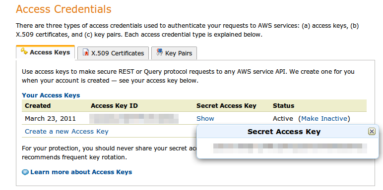
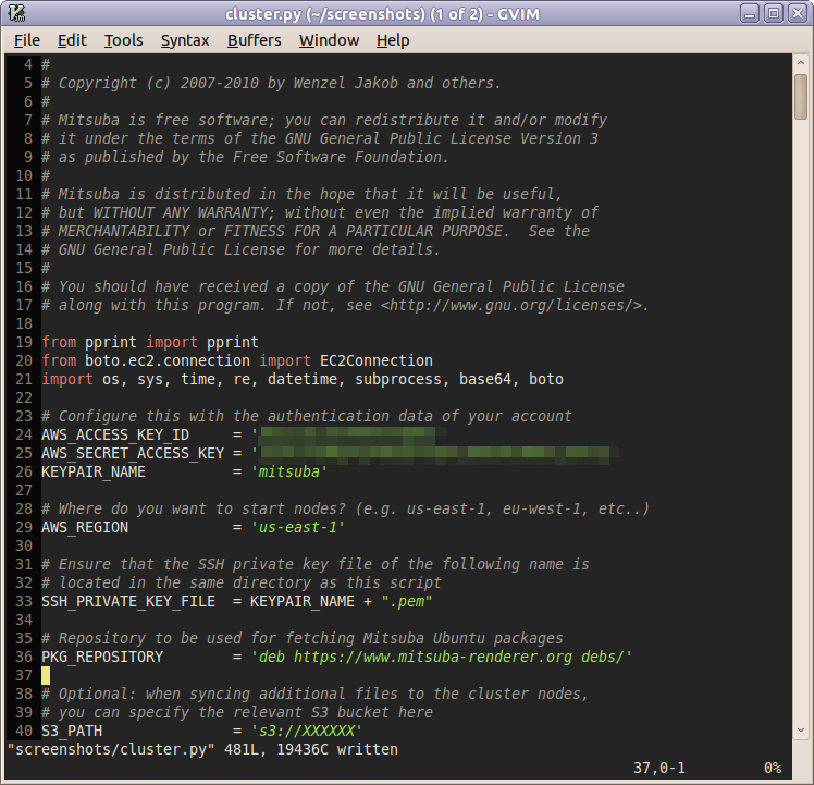
1. After logging into the AWS Management Console, click on “Your Account” and “Security credentials”. Towards the bottom of this page, you should be able to see your Access Key ID, as well as the Secret Access Key. Make note of these two values.
You will need to modify a few values at the top. In particular, the access key, key pair, and region fields all need to be filled out. When building a custom version of Mitsuba, you will also need to modify the PKG_REPOSITORY attribute to point to your own repository.
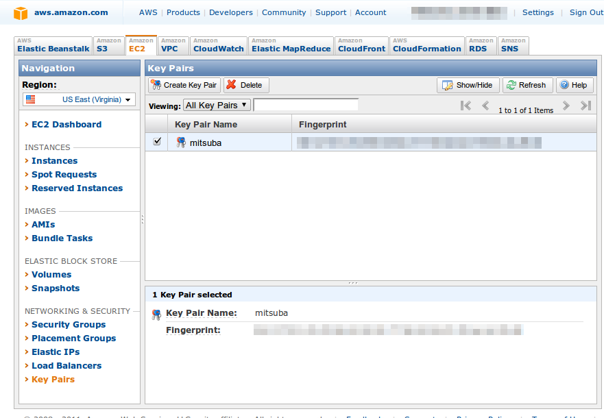
Now, we are almost ready to go. Open a terminal and navigate to the directory containing the modified EC2 launcher script. To set the correct permissions for the private key, execute the following command (replace mitsuba by the name the key pair crated earlier)
$ chmod og-rwx mitsuba.pem
For an overview of all supported commands, type
$ ./cluster.py
The following command allocates a specified number of spot nodes from EC2 and boots them with a stateless version of Ubuntu Maverick (64 bit).
$ ./cluster.py addSpotNodes [instance-type] [count] [bid] <group>
To get an idea of what to specify as a bid, it may be useful to look at the list of previous and current spot prices on the Cloud Exchange. To get (more expensive) regular machines with guaranteed availability, use the following command instead:
$ ./cluster.py addNodes [instance-type] [count] <group>
For instance, to purchase 16 c1.xlarge spot nodes (that’s 128 cores) with a max. bid of $0.30/hr each, enter
$ ./cluster.py addSpotNodes c1.xlarge 16 0.30 myGroup
Requesting 16 spot nodes of type c1.xlarge (group name = "myGroup",
  max. price=0.300)..
Done.
The last parameter designates the name “myGroup” to these 16 machines. To see whether your nodes have started successfully, enter
$ ./cluster.py status
Querying spot instance requests...
  sir-724e8411: status=open, price must be <= 0.300$
  .... (15 more)
When the bid is above the spot price and the requests have been fulfilled (this usually happens within a minute), this status will change to
$ ./cluster.py status
Querying spot instance requests...
  sir-724e8411: status=active, price must be <= 0.300$
  .... (15 more)

Querying instances ...
Nodes in group "myGroup"
===================
  ec2-50-17-103-151.compute-1.amazonaws.com is running (type:
    c1.xlarge, running for: 0d 0h 1m, internal IP: 10.86.31.233,
    spot request: sir-724e8411)
    .... (15 more)
These are perfectly standard Ubuntu machines — to obtain shell access to any one of them, pass the host name seen seen in the previous command to the login command, e.g.
$ ./cluster.py login ec2-50-17-103-151.compute-1.amazonaws.com
To quickly install Mitsuba on all nodes in parallel (time is money at this point!), run
$. /cluster.py install myGroup
Sending command to node ec2-50-17-103-151.compute-1.amazonaws.com
...
0/16 nodes are ready.
...
16/16 nodes are ready.
This process usually takes about 30-60 seconds; a few harmless warnings may appear, which can be ignored. With Mitsuba installed on all machines, the last step is to create a rendering cluster. For this, execute
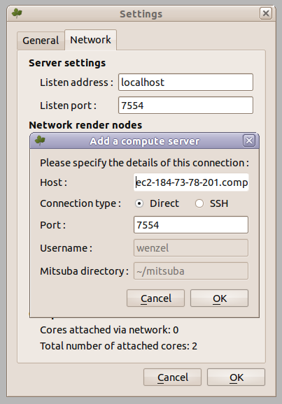
$. /cluster.py start myGroup
Creating a Mitsuba cluster using the nodes of group "myGroup"
Sending command to node ec2-50-17-102-163.compute-1.amazonaws.com
....
15/15 nodes are ready.
All nodes are ready.
Creating head node ..
Done -- you can specify the head node
   "ec2-184-73-78-201.compute-1.amazonaws.com" in the Mitsuba
   network rendering dialog
The host name in this last command is the head node of the cluster. To save network bandwidth, the head node transparently provides access to all cores in the cluster without you having to create internet connections to 16 separate machines.

Default network topology
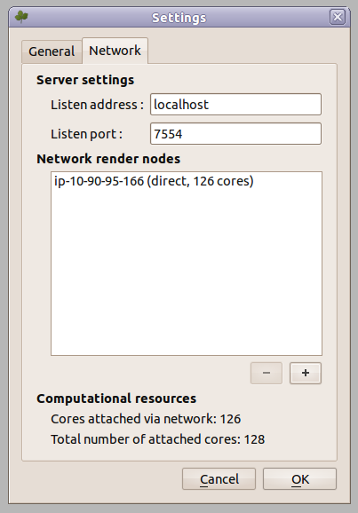
To use the cluster, simply add this machine in the rendering preferences of the Mitsuba GUI or provide it using the -c parameter when rendering from the command line interface.
Once you are done, don’t forget to run
$ ./cluster.py terminateAll myGroup
to shut down the machines and stop any charges to your account (note: Amazon will bill you for any partially used hours).
This guide only covered the most basic use case; more advanced features also supported. For instance, to do some serious rendering with volumetric datasets, I usually upload the (multi-gigabyte) volume data files to Amazon S3 ahead of time. After booting up a cluster, I use the syncData command to have all cluster nodes simultaneously download those files over the EC2-internal network (this does not incur any network charges). Another useful feature is that multiple users can simultaneously create Mitsuba clusters on a single account without interfering, as machines are always referred to using group names.
After a long development cycle, I have just released a new version of Mitsuba. Please read on for a list of changes (these are in addition the ones mentioned in this Blog entry).
Participating Media: the most significant feature of this release is a complete redesign of the participating medium layer in Mitsuba. This change was necessary to remove limitations inherent in the previous architecture, which was overly complicated and could only support a single medium per scene. The new Mitsuba version handles an arbitrary amount of media, which can be “attached” to various surfaces in the scene. For instance, rendering a bottle made of absorbing colored glass now involves instantiating an absorbing medium and specifying that it lies on the interior of the bottle’s glass surface.
Apart from these changes, the new implementations are also significantly more robust, particularly when heterogeneous media are involved. In a future blog post, I will provide more detail on the rewritten participating media layer.
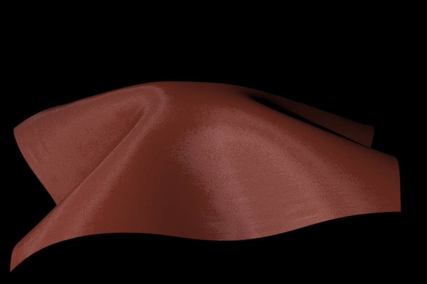
Micro-flake model: Mitsuba was used to create the high-resolution volumetric cloth renderings in the paper “Building Volumetric Appearance Models of Fabric using Micro CT Imaging” by Shuang Zhao, Wenzel Jakob, Steve Marschner, and Kavita Bala.
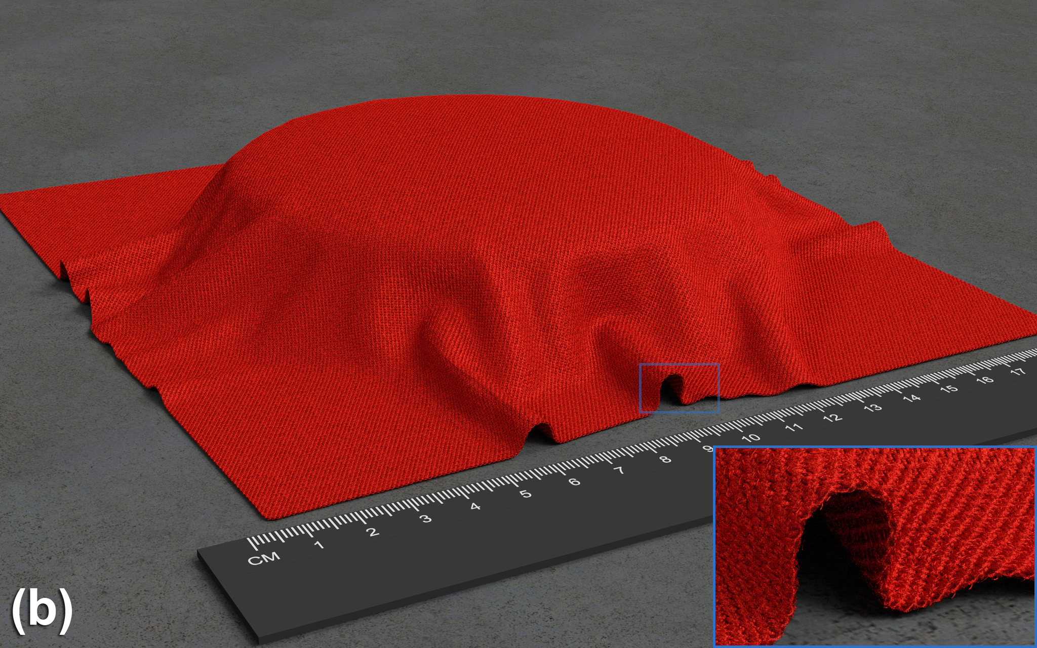
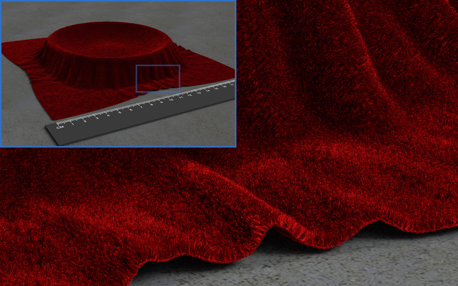
This project was a *big* challenge for the micro-flake rendering code and led to many useful changes. For instance, the code previously made heavy use of spherical harmonics expansions to compute transmittance values, and to importance sample the model. For very shiny materials (such as the cloth models we rendered), this can become a severe problem due to ringing in the spherical harmonics representation. The rewritten model has fast and exact importance sampling code that works without spherical harmonics, and it uses a high-quality numerical approximation for the transmittance function.
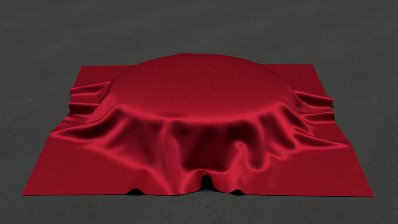
Irawan & Marschner woven cloth BRDF: This release adds a new material model for woven cloth, which was developed by Piti Irawan and Steve Marschner. The code in Mitsuba is a modified port of a previous Java implementation. A few measured patterns shown below are already included as example scenes (many thanks go to Piti for allowing the use of his code and data!)
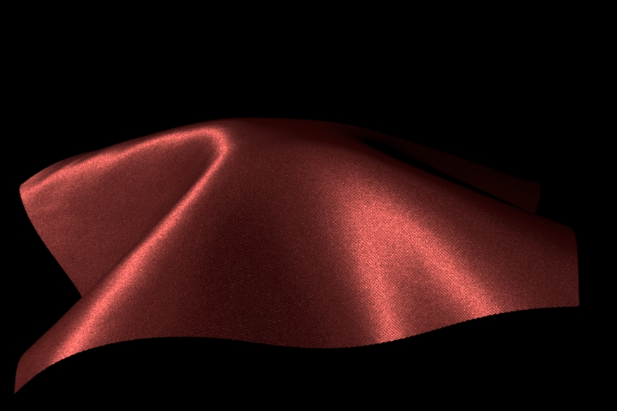


This model relies on a detailed description of the material’s weave pattern, which is described with the help of a simple description language. For instance, the description of polyester lining cloth looks something like the following:
weave {
  name ="Polyester lining cloth",

  /* Weave pattern description */
  pattern {
    3, 2,
    1, 4
  },

  /* Listing of all yarns used in the pattern (numbered 1 to 4) */
  yarn {
    type = warp,
    /* Fiber twist angle */
    psi = 0,
    /* Maximum inclination angle */
    umax = 22,
    /* Spine curvature */
    kappa = -0.7,
    /* Width and length of the segment rectangle */
    width = 1,
    length = 1,
    /* Yarn segment center in tile space */
    centerU = 0.25,
    centerV = 0.25
  },
  ....
}
For more details on this model, please refer to Piti Irawan’s PhD thesis.
Due to its performance and expressiveness, I believe that this model is of genuine utility to a larger audience and hope that including it in Mitsuba will increase its adoption.
A cool feature that I might add in the future is an interactive editor to design new pattern descriptions with a live preview.
Amazon EC2: This release adds a launcher script to create virtual render farms on the Amazon Elastic Compute Cloud (EC2). This is very useful when rendering time is critical, since EC2 can give you essentially infinite parallelism. I will write more on how this works in a separate post.
Blender Plugin: Due to its experimental nature, Blender 2.5x has been a bit of a moving target, making it difficult to develop stable plugins. Recently, a large batch of changes broke many plugins, particularly custom rendering backends. Since then, I have been working on restoring compatibility with Blender 2.56, which is mostly complete at this point. Some work remains to be done, hence I will release the final Blender plugin in a few days.
Build system: The build system has undergone several cleanups:
To upgrade to this version without making a mess of your repository, I recommend to clean before updating, i.e.
$ scons -c
$ hg pull -u
If you forgot that step, old .obj/.os files and other build products will probably litter your source tree. In that case, it might be easiest to check out a clean copy.
If you are on Windows or OSX, note that you must also update the dependencies repository.
Beam Radiance Estimate: Mitsuba now contains an implementation of the Beam Radiance Estimate to accelerate Volumetric Photon Mapping within homogeneous participating media (scene courtesy of Wojciech Jarosz).

COLLADA: Previously, the import of very large scenes using COLLADA failed when the associated XML document contained text nodes that were larger than 10 megabytes. I submitted a patch to fix this in the COLLADA-DOM library, which was recently accepted. Mitsuba now ships with this version of the library.
Rotation Controller: several people commented that the interactive preview navigation was rather unintuitive. I have now added a rotation controller that will be more familiar to people using Maya or Blender. Dragging the mouse while pressing the left button rotates around a fixed point. The right mouse button & mouse wheel move along the viewing direction, and the middle mouse button pans. Press ‘F’ to zoom to the currently selected object and ‘A’ to focus on the whole scene. Note that the previous behavior can still be re-activated through the program preferences.
Miscellaneous: this release adds code to perform adaptive n-dimensional integration (based on the cubature project), as well as a chi-square test for verifying sampling methods. In the future, these will be used to implement an automatic self-test of all scattering models within Mitsuba.
As always, the release also contains a plethora bugfixes, which won’t be listed in detail.
In case you are wondering why this blog suddenly looks so different: I have moved it to WordPress after continuously running into problems with the previous system.
On another note: today or tomorrow, a long-overdue release of Mitsuba will be released. Stay tuned!