Mitsuba Development Blog

Hello all,

much has happened since the last version of Mitsuba, so I figured it’s time for a new official release! I’m happy that were quite a few external contributions this time.

The new features of version 0.5.0 are:

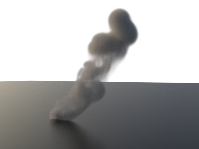
• Multichannel renderings:

  

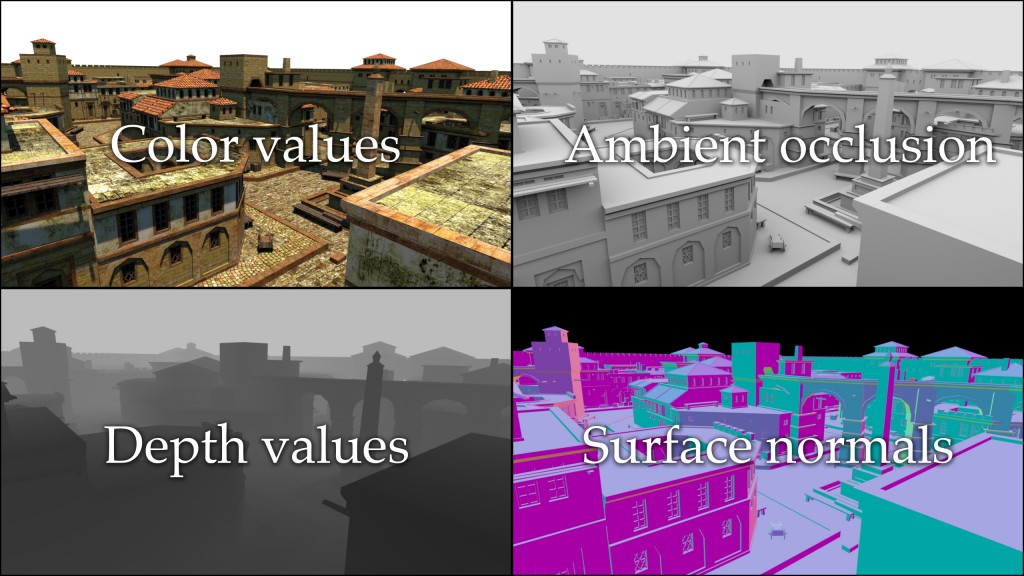
  Mitsuba can now perform renderings of images with multiple channels—these can contain the result of traditional rendering algorithms or extracted information of visible surfaces (e.g. surface normals or depth). All computation happens in one pass, and the output is written to a dense or tiled multi-channel EXR file. This feature should be quite useful to computer vision researchers who often need synthetic ground truth data to test their algorithms. Refer to the multichannel plugin in the documentation for an example.

• Python integration: Following in the footsteps of previous versions, this release contains many improvements to the Python language bindings. They are now suitable for building quite complex Python-based applications on top of Mitsuba, ranging from advanced scripted rendering workflows to full-blown visual material editors. The Python chapter of the documentation has been updated with many new recipes that show how to harness this functionality. The new features include

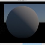
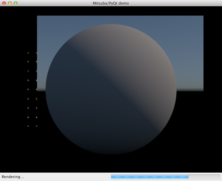
  • PyQt/PySide integration: It is now possible to fully control a rendering process and display partial results using an user interface written in Python. I’m really excited about this feature myself because it will free me from having to write project-specific user interfaces using C++ in the future. With the help of Python, it’s simple and fast to whip up custom GUIs to control certain aspects of a rendering (e.g. material parameters).

    The documentation includes a short example that instantiates and renders a scene while visually showing the progress and partial blocks being rendered. Due to a very helpful feature of Python called buffer objects, it was possible to implement communication between Mitsuba and Qt in such a way that the user interface directly accesses the image data in Mitsuba’s internal memory without the overhead of costly copy operations.

    

  • Scripted triangle mesh construction: The internal representation of triangle shapes can now be accessed and modified via the Python API—the documentation contains a recipe that shows how to instantiate a simple mesh. Note that this is potentially quite slow when creating big meshes due to the interpreted nature of Python.

  • Blender Python integration: An unfortunate aspect of Python-based rendering plugins for Blender is the poor performance when exporting geometry (this is related to the last point). It’s simply not a good idea to run interpreted code that might have to iterate over millions of vertices and triangles. Mitsuba 0.5.0 also lays the groundwork for future rendering plugin improvements using two new features: after loading the Mitsuba Python bindings into the Blender process, Mitsuba can directly access Blender’s internal geometry data structures without having to go through the interpreter. Secondly, a rendered image can be passed straight to Blender without having to write an intermediate image file to disk. I look forward to see these features integrated into the MtsBlend plugin, where I expect that they will improve the performance noticeably.

  • NumPy integration: Nowadays, many people use NumPy and SciPy to process their scientific data. I’ve added initial support to facilitate NumPy computations involving image data. In particular, Mitsuba bitmaps can now be accessed as if they were NumPy arrays when the Mitsuba Python bindings are loaded into the interpreter.

    For those who prefer to run Mitsuba as an external process but still want to use NumPy for data processing, Joe Kider contributed a new feature for the mfilm plugin to write out binary NumPy files. These are much more compact and faster to load compared to the standard ASCII output of mfilm.

  • Python 3.3 is now consistently supported on all platforms

  • On OSX, the Mitsuba Python bindings can now also be used with non-Apple Python binaries (previously, doing so would result in segmentation faults).

• GUI Improvements:
  
  

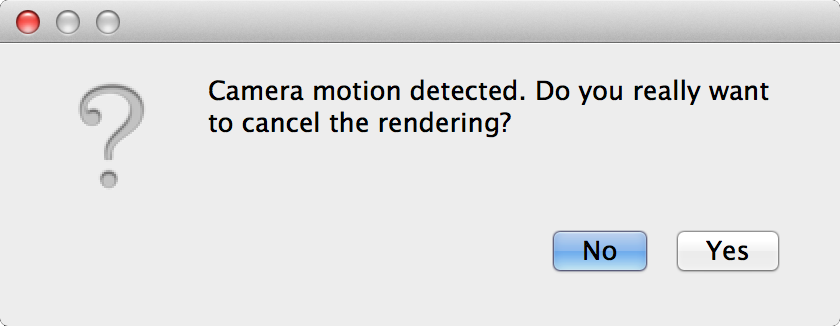
  • Termination of rendering jobs: This has probably happened to every seasoned user of Mitsuba at some point: an accidental click/drag into the window stops a long-running rendering job, destroying all progress made so far. The renderer now asks for confirmation if the job has been running for more than a few seconds.

    
    

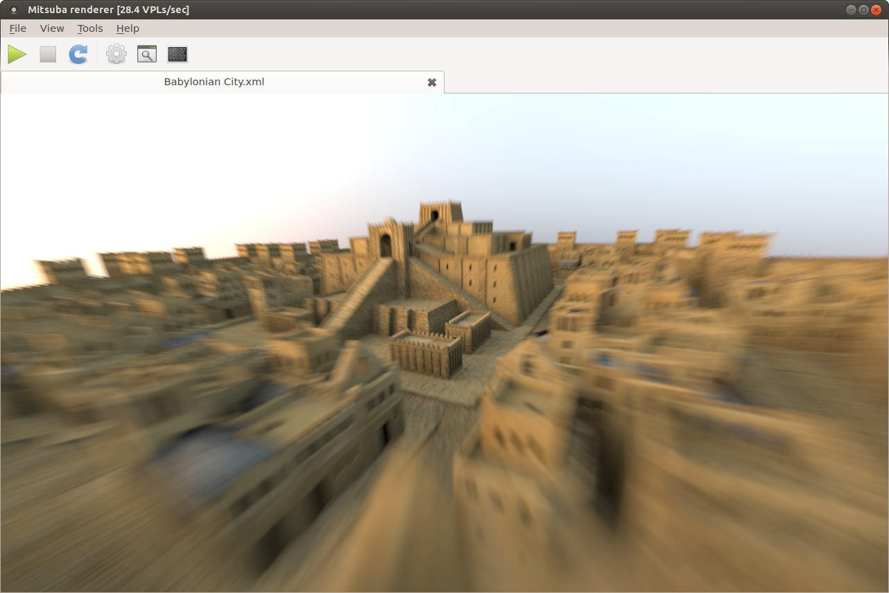
  • Switching between tabs: The Alt-Left and Alt-Right have been set up to cycle through the open tabs for convenient visual comparisons between images.

  • Fewer clicks in the render settings: Anton Kaplanyan contributed a patch that makes all render settings fields directly editable without having to double click on them, saving a lot of unnecessary clicks.

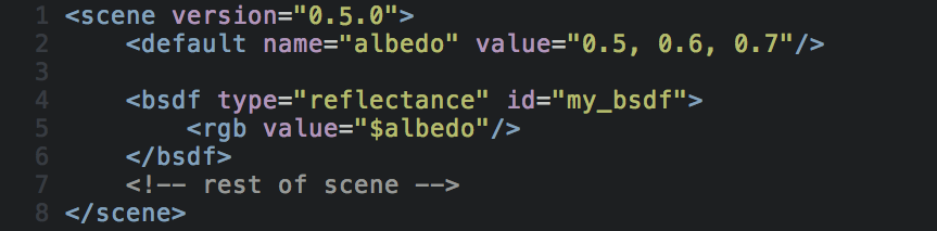
• New default tag: One feature that has been available in Mitsuba since the early days was the ability to leave some scene parameters unspecified in the XML description and supply them via the command line (e.g. the albedo parameter in the following snippet). This is convenient but has always had the critical drawback that loading fails with an error message when the parameter is not explicitly specified. Mitsuba 0.5.0 adds a new XML tag named default that denotes a fallback value when the parameter is not given on the command line. The following example illustrates how to use it:
  

  

• Windows 8.x compatibility: In a prior blog post, I complained about running into serious OpenGL problems on Windows 8. I have to apologize since it looks like I was the one to blame: Microsoft’s implementation is fine, and it was in fact a bug in my own code that was causing the issues. With that addressed in version 0.5.0, Mitsuba now also works on Windows 8.

• CMake build system: The last release shipped with an all-new set of dependency libraries, and since then the CMake build system was broken to the point of being completely unusable. Edgar Velázquez-Armendáriz tracked down all issues and submitted a big set of patches that make CMake builds functional again.

• Other bugfixes and improvements: Edgar Velázquez-Armendáriz fixed an issue in the initialization code that could lead to crashes when starting Mitsuba on Windows

  The command line server executable mtssrv was inconvenient to use on Mac OS X because it terminated after any kind of error instead of handling it gracefully. The behavior was changed to match the other platforms.

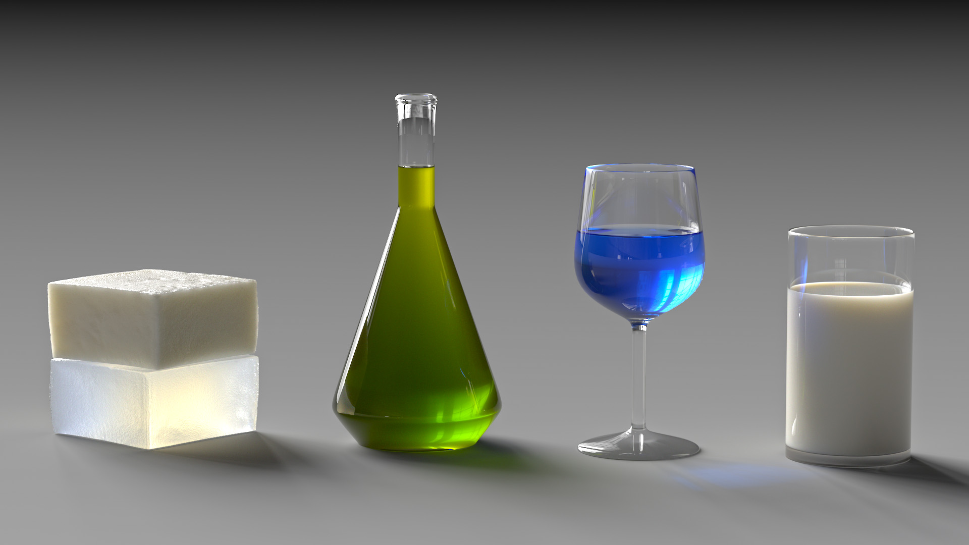
  A previous release contained a fix for an issue in the thin dielectric material model. Unfortunately, I did not apply the correction to all affected parts of the plugin back then. I’ve since then fixed this and also compared the model against explicitly path traced layers to ensure a correct implementation.

  Anton Kaplanyan contributed several MLT-related robustness improvements.

  Anton also contributed a patch that resets all statistics counters before starting a new rendering, which is useful when batch processing several scenes or when using the user interface.

  Jens Olsson reported some pitfalls in the XML scene description language that could lead to inconsistencies between renderings done in RGB and spectral mode. To address this, the behavior of the intent attribute and spectrum tag (for constant spectra) was slightly adapted. This only affects users doing spectral renderings, in which case, you may want to take a look at Section 6.1.3 of the new documentation and the associated entry on the bug tracker.

I’d also like to announce two new efforts to develop plugins that integrate Mitsuba into modeling applications:

• Rhino plugin: TDM Solutions SL published the first version of an open source Mitsuba plugin for Rhino 3D and Rhino Gold. The repository of this new plugin can be found on GitHub, and there is also a Rhino 3D group page with binaries and documentation. It is based on an exporter I wrote a long time ago but adds a complete user interface with preliminary material support. I’m excited to see where this will go!

• Maya plugin: Jens Olsson from the Volvo Car Corporation contributed the beginnings of a new Mitsuba integration plugin for Maya. Currently, the plugin exports geometry to Mitsuba’s .serialized format but still requires manual XML input to specify materials. Nonetheless, this should be quite helpful for Mitsuba users who model using Maya. The source code is located in the mitsuba-maya repository and prebuilt binaries are here.

Getting the new version

Precompiled binaries for many different operating systems are available on the download page. The updated documentation file (249 pages) with coverage of all new features is here (~36 MB), and a lower resolution version is also available here (~6MB).

By the way: a little birdie told me that Mitsuba has been used in a bunch SIGGRAPH submissions this year. If all goes well, you can look forward to some truly exciting new features!

My fiancée baked some Mitsuba leaf-shaped Christmas cookies.

To cut them out of the dough, she 3D-printed the logo into wax and cast it into silver.

Awesome!

Hello all,

I’m happy to release a new version of Mitsuba containing many bugfixes and a couple of new features. They are as follows:

• Height field intersection shape:
  
  
  
  The heightfield primitive represents a quad that is vertically displaced by an arbitrary texture. All storage and ray intersection computations are done in image space (i.e. without creating explicit dense triangle geometry), which leads to significantly better performance. This new plugin was contributed by Miloš Hašan and adapted by Wenzel Jakob. Internally, it relies on the Min-Max MIP Map acceleration data structure.

• Perspective camera model with radial distortion:

  When rendering images that are supposed to look just like an image taken by a real-world camera, it is important to take lens distortions into account. Mitsuba now has a new perspective_rdist plugin that accepts fitted radial distortion parameters from standard camera calibration packages like the MATLAB Camera Calibration toolbox by Jean-Yves Bouguet.

• Fast image convolution & bloom filter:

  Mitsuba now supports fast convolutions of large 2D images in frequency space using a convolution theorem approach (Fourier Transform implemented via the FFTW library). This is a pretty standard technique, though it sometimes seems like magic.

  This fast convolution method used to implement Spencer et al’s physically-based bloom filter in the mtsutil tonemap utility. This can be useful when rendering images where pixels are clipped because they are so bright. Take for instance the rendering below: there are many reflections of the sun, but they are quite hard to perceive due to the limited dynamic range. After convolving the image with an empirical point spread function of the human eye, their brightness is much more apparent.
  

  
  
  

• Initial Retina display support, support for OSX 10.8:

  The latest iteration of OSX and Apple’s new devices with HiDPI monitors brought countless changes that caused problems with the last version of Mitsuba. This release addresses many of them, though full HiDPI support will still have to wait until Digia fixes several critical OSX-related bugs in Qt5.

• Texture channel filter:

  The bitmap texture has a new feature to create a grayscale texture from a specified bitmap channel (e.g. alpha). This is useful in conjunction with the mask plugin.

• Python bindings:

  Considerably expanded Python binding coverage and better support for recent Python releases. The Windows package now comes with bindings for versions 2.7, 3.2, and 3.3; all Linux packages come with bindings for the Python 2.x and 3.x releases of the respective distributions.

  This release also adds convenience functions for quickly converting between Mitsuba bitmaps and Python bytearray data structures. This can be useful when shuffling data between Python binding libraries, such as Mitsuba and PyQt/PySide.

• Multithreading:

  By default, Mitsuba collects lots of statistics while rendering a scene. A key requirement for this process is that it should not impact rendering time in any significant way, and the implementation tries to ensure that this is indeed the case. For instance, to prevent resource contention involving performance counters, Mitsuba replicates them many times so that each thread has access to a unique uncontended memory region.

  As it turns out, this replication was not quite working as expected, causing slowdowns on machines with many cores (e.g. >4). This problem has been fixed.

  Another threading-related change that has brought small but measurable performance improvements is that worker threads now request CPU affinity on platforms where this is supported (Windows and Linux).

• Visual Studio 2013 support:

  As of about a month ago, the new version of Visual Studio is available. Those who develop on Windows will be pleased to hear that it’s now possible to work on Mitsuba using this compiler—also, all pesky compilation of dependencies has been done for you. The older visual Studio 2010 will continue to be supported in the future.

  To get the most recent version of SCons to work with Visual Studio 2013, a small modification to the SCons code is necessary: change lines 132+ in the file scons-2.3.0\SCons\Tool\MSCommon\vc.py so that they read

  _VCVER = ["12.0", "11.0", "11.0Exp", "10.0", ...
  _VCVER_TO_PRODUCT_DIR = {
      '12.0': [
          r'Microsoft\VisualStudio\12.0\Setup\VC\ProductDir'],
      '11.0': [
          r'Microsoft\VisualStudio\11.0\Setup\VC\ProductDir'],

  and so on.

• New dependency binaries:

  For consistency, all dependency binaries have been brought up to date on Windows and Mac OS X.

• KD-tree improvements when rendering in double precision:

  Due to roundoff errors when converting between single and double precision, faces that were aligned with the top-level bounding box of a kd-tree could get clipped. This caused problems when rendering in double precision, particularly when using the instance plugin.

• Many smaller robustness fixes and bugfixes in various parts of the renderer—see the repository for details.

I’ll close with a link to an interesting paper which tackles an extremely difficult measurement problem, to be presented at SIGGRAPH Asia next week. The paper’s teaser image was rendered using the volumetric path tracer in Mitsuba.

• Inverse Volume Rendering with Material Dictionaries (by Ioannis Gkioulekas, Shuang Zhao, Kavita Bala, Todd Zickler, and Anat Levin)
  
  
  
  Abstract: Translucent materials are ubiquitous, and simulating their appearance requires accurate physical parameters. However, physically-accurate parameters for scattering materials are difficult to acquire. We introduce an optimization framework for measuring bulk scattering properties of homogeneous materials (phase function, scattering coefficient, and absorption coefficient) that is more accurate, and more applicable to a broad range of materials. The optimization combines stochastic gradient descent with Monte Carlo rendering and a material dictionary to invert the radiative transfer equation. It offers several advantages: (1) it does not require isolating single-scattering events; (2) it allows measuring solids and liquids that are hard to dilute; (3) it returns parameters in physically-meaningful units; and (4) it does not restrict the shape of the phase function using Henyey-Greenstein or any other low-parameter model. We evaluate our approach by creating an acquisition setup that collects images of a material slab under narrow-beam RGB illumination. We validate results by measuring prescribed nano-dispersions and showing that recovered parameters match those predicted by Lorenz-Mie theory. We also provide a table of RGB scattering parameters for some common liquids and solids, which are validated by simulating color images in novel geometric configurations that match the corresponding photographs with less than 5% error.

Things have been a little quiet around here as of late. Writing my thesis, finishing course work, and moving to another country all took a toll on the amount of time left for Mitsuba coding. So I am happy to say that I’ve finally moved, graduated from Cornell, and just turned in my Ph. D. thesis!

It’s called Light Transport on Path-Space Manifolds and is essentially a significantly expanded version of the Manifold Exploration paper (from 13 to 153 pages).

If you’re interested, click below for a link to the full thesis (20MB PDF).

Hello all,

I’ve uploaded binaries for the Mitsuba 0.4.4 release. This is mainly a bugfix release to address issues concerning the previous version. There is, however, one new feature:

Improved Python bindings for rendering animations

It’s a fairly common operation to render a turntable animation of an object to understand its shape a little better. So far, doing this in Mitsuba involved many separate invocations of the renderer (one for each frame). Not only is this a bit tedious, but it also wastes a considerable amount of CPU time by loading and preprocessing the same scene over and over again. Python to the rescue!

In Mitsuba 0.4.4, the Python bindings make this kind of thing straightforward: simply load the scene and render out frames in a for loop. The following piece of code does this, together with motion blur. The work can be spread over the local cores or those on networked machines. Some setup code is omitted for brevity (see the Python chapter in the documentation for all details).

# Render a turntable with 360 / 2 = 180 frames
stepSize = 2
for i in range(0,360 / stepSize):
    # Compute the rotation at the beginning and the end of the frame
    rotationCur  = Transform.rotate(Vector(0, 0, 1), i*stepSize);
    rotationNext = Transform.rotate(Vector(0, 0, 1), (i+1)*stepSize);

    # Compute matching camera-to-world transformations
    trafoCur  = Transform.lookAt(rotationCur  * Point(0,-6,10),
        Point(0), rotationCur  * Vector(0, 1, 0))
    trafoNext = Transform.lookAt(rotationNext * Point(0,-6,10),
        Point(0), rotationNext * Vector(0, 1, 0))

    # Create an interpolating animated transformation
    atrafo = AnimatedTransform()
    atrafo.appendTransform(0, trafoCur)
    atrafo.appendTransform(1, trafoNext)
    atrafo.sortAndSimplify()
    sensor.setWorldTransform(atrafo) # Assign to the sensor

    # Submit the frame to the scheduler and wait for it to finish
    scene.setDestinationFile('frame_%03i.png' % i)
    job = RenderJob('job_%i' % i, scene, queue)
    job.start()
    queue.waitLeft(0)
    queue.join()

This is basically a 1:1 mapping of the C++ API. At this point, a good amount of the interfaces have been exposed, making it fun to prototype stuff while subjected to the amazing weightlessness of Python. Here, you can see an example of a video created this way (a turntable of the material test ball with a bumpy metal BSDF):

Other changes

• Photon mapper: In previous releases, the standard photon mapper could miss certain specular paths compared to the path tracer. They are now correctly accounted for.

• thindielectric: The thindielectric plugin computed incorrect transmittance values in certain situations; this is now fixed.

• Robustness: Improved numerical robustness when dealing with specular+diffuse materials, such as “plastic”.

• twosided: Fixed cases where the twosided plugin did not make a material two-sided as expected.

• Instancing: The shading computed shading frame was incorrect for non-rigid transformations.

• Cube shape: This recently added shape is now centered at the origin by default, to be consistent with the way that other shapes in Mitsuba work. This will require an extra translation in scenes which are already using the cube shape.

• TLS cleanup logic: on some platforms, the mtssrv binary crashed with an exception after finishing a rendering job, due to some issues with cleaning up thread-local storage.

• Other minor fixes and improvements, which are listed in the HG history

Hello all,

I’ve just uploaded binaries for a new version of Mitsuba. This release and the next few ones will focus on catching up with a couple of more production-centric features. This time it’s motion blur — the main additions are:

Moving light sources

The first image below demonstrates a moving point light source in a partially metallic Cornell box moving along a Rose curve. Because it’s rendered with a bidirectional path tracer, it is possible to see the actual light source. Due to the defocus blur of the camera, the point light shows up as a ribbon instead of just a curve.

This can be fairly useful even when rendering static scenes, since it enables building things like linear light sources that Mitsuba doesn’t natively implement.
Animating a light source is as simple as replacing its toWorld transformation

<transform name="toWorld">
 ... emitter-to-world transformation ...
</transform>

with the following new syntax

<animation name="toWorld">
   <transform time="0">
     ... transformation at time 0 ...
   </transform>

   <transform time="1">
     ... transformation at time 1 ...
   </transform>
</animation>

Mitsuba uses linear interpolation for scaling and translation and spherical linear interpolation for rotation. Higher-order interpolation or more detailed animations can be approximated by simply providing multiple linear segments per frame.

Moving sensors

Moving sensors work exactly the same way; an example is shown below. All new animation features also provide interactive visualizations in the graphical user interface (medieval scene courtesy of Johnathan Good).

Rendering

Interactive preview

Objects undergoing linear motion

Objects can be animated with the same syntax, but this is currently restricted to linear motion. I wanted to include support for nonlinear deformations in this release, but since it took longer than expected, it will have to wait until the next version.

Render-time annotations

The ldrfilm and hdrfilm now support render-time annotations to facilitate record keeping. Annotations are used to embed useful information inside a rendered image so that this information is later available to anyone viewing the image. They can either be placed into the image metadata (i.e. without disturbing the rendered image) or “baked” into the image as a visible label. Various keywords can be used to collect all relevant information, e.g.:

 <string name="label[10, 10]" value="Integrator: $integrator['type'],
   $film['width']x$film['height'], $sampler['sampleCount'] spp,
   render time: $scene['renderTime'], memory: $scene['memUsage']"/>

Providing the above parameter to hdrfilm has the following result:

Hiding directly visible emitters

Several rendering algorithms in Mitsuba now have a feature to hide directly visible light sources (e.g. environment maps or area lights). While not particularly realistic, this feature is convenient for removing a background from a rendering so that it can be pasted into a differently-colored document. Together with an improved alpha channel computation for participating media, things like the following are now possible:

Original image

Composited onto a white background

Improved instancing

While Mitsuba has supported instancing for a while, there were still a few lurking corner-cases that could potentially cause problems. In a recent paper on developing fractal surfaces in three dimensions, Geoffrey Irving and Henry Segerman used Mitsuba to render heavy scenes (100s of millions of triangles) by instancing repeated substructures— this was a good incentive to fix the problems once and for all. The revamped instancing plugin now also supports non-rigid transformations. The two renderings from the paper shown below illustrate a 2D Gospel curve developed up to level 5 along the third dimension:

Top view

Bottom view

Miscellaneous

• Threading on Windows: Edgar Velázquez-Armendáriz fixed the thread local storage (TLS) implementation and a related race condition that previously caused occasional deadlocks and crashes on Windows

• Caching: Edgar added a caching mechanism to the serialized plugin, which significantly accelerates the very common case where many shapes are loaded from the same file in sequence.

• File dialogs: Edgar upgraded most of the “File/Open”-style dialogs in Mitsuba so that they use the native file browser on Windows (the generic dialog provided by Qt is rather ugly)

• Python: The Python bindings are now much easier to load on OSX. Also, in the new release, further Mitsuba core functions are exposed.

• Blender interaction: Fixed a issue where GUI tabs containing scenes created in Blender could not be cloned

• Non-uniform scales: All triangle mesh-based shapes now permit non-uniform scales

• NaNs and friends: Increased resilience against various numerical corner cases

• Index-matched participating media: Fixed an unfortunate regression in volpath regarding index-matched media that was accidentally introduced in 0.4.2

• roughdiffuse: Fixed texturing support in the roughdiffuse plugin

• Photon mapping: Fixed some inaccuracies involving participating media when rendered by the photon mapper and the Beam Radiance Estimate

• Conductors: Switched Fresnel reflectance computations for conductors to the exact expressions predicted by geometric optics (an approximation was previously used)

• New cube shape: Added a cube shape plugin for convenience. This does exactly what one would expect.

• The rest: As usual, a large number of smaller bugfixes and improvements were below the threshold and are thus not listed individually—the repository log has more details.

Where to get it

The documentation was updated as well and has now grown to over 230 pages. Get it here.
The new release is available on the download page

The next bug-fix release of Mitsuba is available, which has the following improvements:

• Volumetric path tracers: improved sampling when dealing with index-matched medium transitions. This is essentially a re-implementation of an optimization that Mitsuba 0.3.1 already had, but which got lost in the bidirectional rewrite.

• Batch tonemapper: due to an unfortunate bug, the batch tonemapper in the last release produced invalid results for images containing an alpha channel. This is now fixed.

• Shapes: corrected some differential geometry issues in the “cylinder” and “rectangle” shapes.

• MLT: fixed 2-stage MLT, which was producing incorrect results.

• MEPT: fixed the handling of directional light sources.

• Robustness: got rid of various corner-cases that could produce NaNs.

• Filenames: to facilitate loading scenes created on Windows/OSX, the Linux version now resolves files case-insensitively if they could not be found after a case-sensitive search.

• Python: added Python bindings for shapes and triangle meshes. The Python plugin should now be easier to load (previously, this was unfortunately rather difficult on several platforms). The documentation was also given an overhaul.

• Particle tracing: I’ve decided to disable the adjoint BSDF for shading normals in the particle tracer, since it causes an unacceptable amount of variance in scenes containing poorly tesselated geometry. This affects the plugins ptracer, ppm, sppm and photonmapper. See the commit for further details.

• Subsurface scattering: fixed parallel network renderings involving the dipole model.

• Homogeneous medium & dipole: added many more material presets by Narasimhan et al.

• OBJ loader: further robustness improvements to the OBJ loader and the associated MTL material translator.